Piecing Together the Puzzle of Property Prices with Peer-to-Peer Lending Data

Data science provides a venue that exercises the inquisitive mind. The opportunity to investigate new datasets and understand their value for a theory or model never ceases to fascinate and enthral.
That inquisitive nature — the mission to understand what drives value in the commercial real estate (CRE) market — runs at the core of what we do here at GeoPhy. It leads to the exploration and analysis of a wide variety of data. This variety and the unprecedented volume of data now available provide two of the conventional “V’s” of big data [1], and make this quest both a compelling and complicated one — like fitting together pieces of a puzzle.
Puzzle pieces
At GeoPhy, we’ve developed an Automated Valuation Model (AVM) in which building income naturally reflects a significant determining value factor for commercial real estate. However, building income can be challenging to directly or consistently secure across time and space. Yet without it, we miss vital pieces of the data puzzle. That leaves us faced with the mission of identifying alternative pieces that fit (read: sufficiently approximate) the “income-shaped” hole in our puzzle.
For multifamily residential buildings, which represent a significant component of the CRE space, household income often reflects rental price thresholds. Thus identifying indicators of household financial health, with the intuition that they have an important relationship with residential building income such as rent, provides a reasonable strategy (there are many others of course). But does data exist to support that strategy? One dataset we’ve recently turned to is loan statistics from a major peer-to-peer lending organization, Lending Club.
Loan data
Lending Club (LC) is a peer-2-peer (P2P) lending service. P2P services match individuals who need to borrow money (e.g., to finance a car or consolidate credit card debt) with individuals willing to lend money without an intermediary institution (i.e., bank). Breakthroughs in technology have allowed this form of financing to grow considerably [2], [3]. In addition to providing the platform technology for this exchange, P2P services set a credit policy for underwriting the loans, and some make the data they use in their due diligence available publicly to reduce information asymmetry that arises when lenders do not have access to enough information about the borrowers.
Lending Club provides data on all successful loan applications, both current and closed, as well as rejected applications. Records of successful loans contain dozens of attributes about the loan such as loan amount, issue date, interest rate, a category and loan purpose description, loan status, and so on. These records also provide attributes about the borrower, which include credit history, reported income, whether they own or rent, number of years employed and so on. Lending Club anonymizes the loan data provided to prevent identification of personal information. From that data, we extract a time series with unit resolution of month and “regional zip-code area” (zips sharing a 3-digit prefix, the most granular location information provided). This dataset goes back to 2007 and is updated quarterly. As of August 2018, there were ~2 million successful loan applications and ~22 million failed applications.
Some interesting research has looked at this data [4]. It has also been the subject of a Kaggle competition. While previous work has focused on predicting loan defaults using the loan dataset itself, GeoPhy looks at incorporating loan data as a proxy for financial conditions and a factor in property values within a more complex model.
Analyzing time series data presents some interesting technical challenges, and while much of that is out of scope for this post, we’ll reference it as we focus on a brief overview of our exploratory data analysis.
A statistical deep-dive into Lending Club data
A quick look at distribution plots of a few key variables provides some valuable insights into the data.
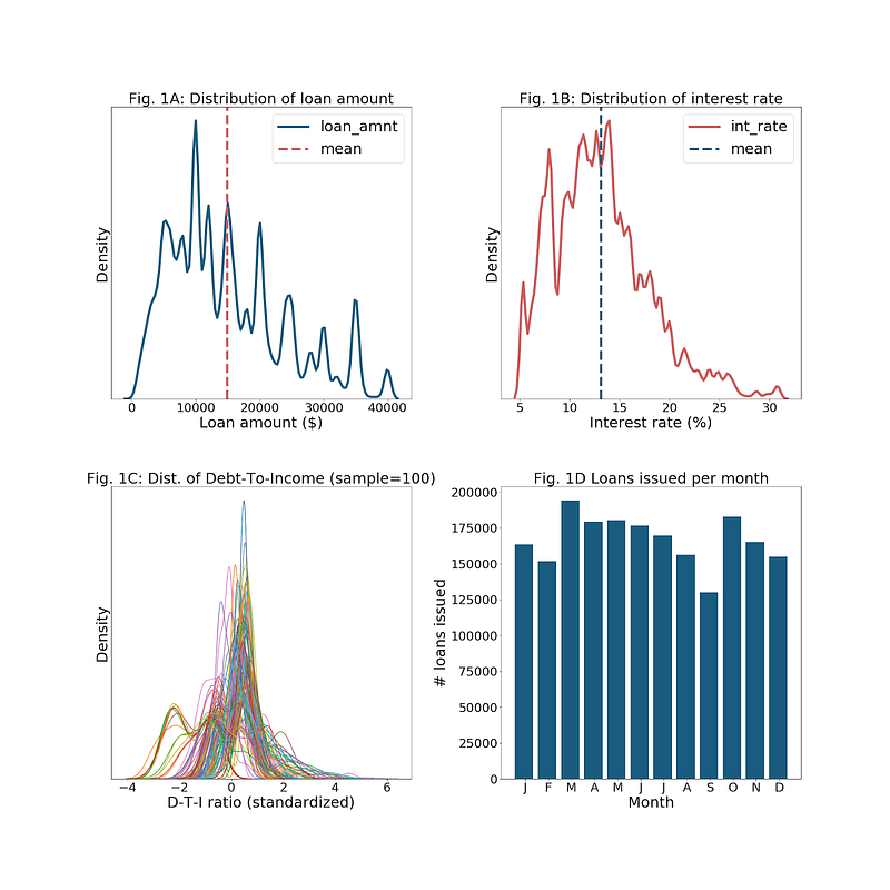
Figure 1 (above):
1A) We see a multinomial distribution of loan amounts, with the greatest concentration at $10K, mean of ~$15K and strong tendencies around roughly $5K increments up to $40K;
1B) Interest rates are densest around 7% and between 11–15%, with mean ~13%, and then drop (of course, these high-interest rates reflect the risk of the peer-to-peer loans!);
1C) There is variance and some distinction around the ratio of debt-to-income across zip-code groups; and
1D) Loans per month show some seasonality (Christmas debt, as well as money spent during or for Summer vacations, appear to be refinanced after 90 days).
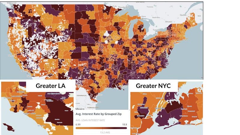
Figure 2 (above): Variance across zip-code groups is evident spatially when viewing interest rates by zip-code group on a map, particularly the zoomed insets of LA and NYC.
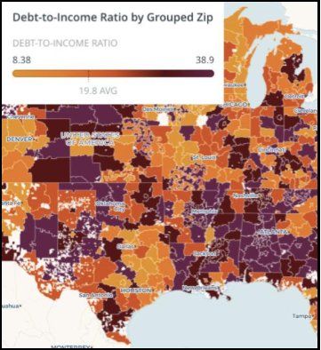
Figure 3: Mapping debt-to-income ratios reveals that many small- to mid-size cities throughout the Midwest appear to have different debt-to-income ratios than the suburban areas immediately surrounding them — a relationship that may inform building value.
We have to be careful to identify assumptions and constraints in the data, such as Lending Club policy or regulatory impacts. For example, borrowers in the state of Iowa are not currently able to use Lending Club — something that can be readily observed in the data. It’s also critical to identify endogenous factors, such as a trend in the overall volume of loans due to growth in Lending Club’s popularity as a service, not some change in borrower behavior.
Investigating data structure
While we don’t mean to focus on time series analysis with this post, it is important to note the availability of other data processing methods that can be useful for identifying structure that signals important information versus noise. Standardizing the data as well as using ARIMA (autoregressive integrated moving average) models can help.
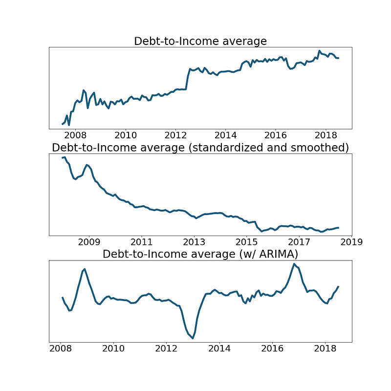
Figure 4 (above): We see the impact of feature transformation on the average debt-to-income ratio across all records. The top graph illustrates the raw average ratio. In the middle, cross-sectional standardization (zero-mean, unit variance) mitigates the upward trend that appears to be global (perhaps due to Lending Club’s growing popularity among risker borrowers?), and a Gaussian filter (0.5 sigma) smooths the data. At the bottom, we applied ARIMA (6-month lag and moving avg.), which highlights aberrations in the time series, such as the uptick in late 2008/early 2009, the downtick in 2013, and another uptick in 2017.
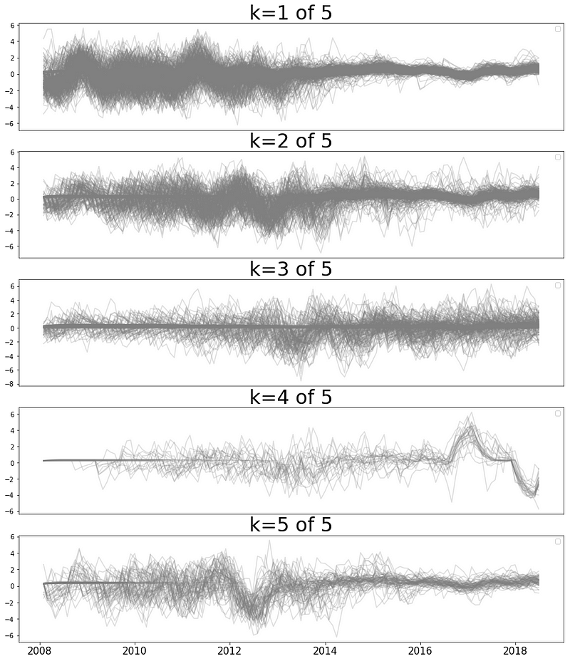
Figure 5 (above): Clustering also reveals interesting structure. These plots represent average interest rates after applying ARIMA and clustered with an agglomerative clustering algorithm to discover distinct patterns.
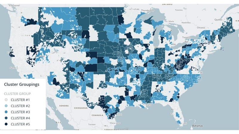
Figure 6 (below): When plotted on a map, these groups revealed more information about the data. For example, there are clearly state-level factors affecting interest rates as can be seen prominently in cluster #4 and somewhat in other clusters. Contrast these state forms with the overall average interest rates in the map above, which were mapped with the exact same geographical boundaries. It is interesting to note the distinct fluctuation of interest rates in cluster #4 above in 2016 and later, potentially indicating state-level events such as changes in regulation or Lending Club policy.
Identifying loan to building income relationships
We began investigation of Lending Club data to explore how loan data informs building value. As initial clustering has indicated, there appears to be some temporal and spatial structure to loan data that may prove valuable for the AVM. Recall, our initial strategy was to identify possible relationships with loan data and building income.

Figure 7: When comparing the known “net operating income” (NOI) of some buildings in GeoPhy’s database with the average interest rate of Lending Club borrowers in the state, there does indeed appear to be a statistically significant relationship — e.g., as average interest rates increase, the NOI per building unit decreases.
Future work
Upon initial analysis, it appears to be a dataset worth looking into further to better grasp how loan data may inform building value. Digging into the temporal nature of this data could provide further relevant insights. What if we looked at loan data for an area around a building leading up to its sale to see if loan data could provide any leading indication of building income or value? Are there cycles in the economic behavior of borrowers that in any way inform the growth of an area or the value of its buildings?
Caveats abound. For example, there are a limited sample of loans available for the time period buildings in our portfolio were sold. That sample may not be representative of the entire universe of Lending Club loan data. Furthermore, there is no certainty the Lending Club dataset itself reflects an appropriate proxy for household financial health. It’s also important to note that our strategy introduces a second-order estimation that compounds errors: the first-order uncertainty relates to our premise that income is a good indicator of building value and the second-order relates to uncertainty of how well loan data informs building income.
Understanding these assumptions and uncertainties is part of the data scientist’s job — an increasingly critical one as the world gets flooded with ever-more disparate data sources. Raw information is a resource that, when carefully cultivated, can yield benefits. A principal aim of GeoPhy’s work is to bring transparency to a large and relatively opaque aspect of our economy — commercial real estate transactions. As we do that, investigating data sources such as loan data, will hopefully bring meaning and value to more pieces in the puzzle.